Primary Market

• Primary market
• Elastic supply curve
  • Maximally available capacity
  • Contra indication of elasticity
• Bidders
  • Aggregation of demand
• Improving the typical Allocation rule
  • Ensuring Alpha Lottery blocks
  • Bidder characteristics
• Relation to the secondary market
  • Important Mechanism Side Effects

Primary market

The Primary Market refers to the Permissioned Call Market. This is the market where the auction for β beta blockspace.

The Call Market is implemented as an Augmented Uniform Price Auction.

We are augmenting the standard uniform price auction format with two features:

1. Instead of providing a perfectly inelastic supply (also known as a fixed amount that we auction off), we offer an elastic supply schedule: If the price is very low, we will offer only limited amounts of options.

2. We introduce a different tie-breaking rule for excess demand. Owing to the discrete nature of bids, situations can arise where no market-clearing price exists (where demand equals supply). While the typical rule in many auctions prioritizes high marginal bids first, we propose an alternative that exerts more pressure at the marginal quantity level.

Elastic supply curve

• Fix the max capacity of beta, $q^{max}$. We assume this is given for the auction. Obviously, it can be a parameter that we will optimize over time.

• The supply curve, $S \colon P \to Q$, where $P$ is the set of allowed prices; and $Q$ the set of available options. It gives for each price the amount of gas space we offer.

• The set of options will be determined by the tick size we provide. $Q$ will be further limited by the max capacity we offer. That is, typically, $Q=\{0,t_q,2t_q,..,q^{max}\}$ where $t_q$ is the tick size of one option and it should hold

Maximally available capacity

$$t_q=q^{max}/k$$

for some $k \in N$.

• The idea for the shape of the supply function is to have an initial segment of the supply curve which is concave and a second segment that then only provides a constant amount.

  note

  This is the maximally available capacity.

Concretely, one parameterized functional form is this:

$$S(p) = \begin{cases} s(p) & \text{for } p < p' \\ s(p') & \text{for } p >= p' \end{cases}$$

where $s(p)$

$$s(p) = ap^n$$

where $a,n$ are constants.

The idea, again, is that the function is concave and thereby monotonically increasing until price $p'$.

This price is calculated by setting the max quantity, $q^{max} = ap^n$, and then deriving

$$p' \equiv (q^{max} / a)^{1/n}$$

warning

The functional form above is up for change depending on the results of the auction.

Contra indication of elasticity

It is theoretically well understood that an elastic supply curve can reduce the danger of dramatically underpricing. In practice, this is not so often used. One reason can be that the value of the good might be lower for the auctioneer.

In our case, however, this can be different. The reason is that we possibly have use for the space ourselves. So, as remarked above, we might have a positive outside value and might not be willing to sell for any price.

Bidders

Each bidder can submit several $(quantity,price)$ pairs. We thereby elicit their partial demand function $d_i(p) \colon P \to Q$.

Aggregation of demand

The way that a uniform auction proceeds is by aggregating demand and matching it to supply. This allows to determine a market clearing price - if it exists.

tip

Reasons for non-existence can be increasing demand curves.

Now, first, consider the aggregate demand:

$$D(p) \equiv \sum_j d_j(p)$$

Fix the highest price at which the all the demand can be satisfied (if it exists). That is,

$$p^{*}=max\{p|D(p)=S(p)\}$$

In the case where there is excess demand for this price, i.e. $D(p^{*})>S(p^{*})$, we need an allocation rule that determines who gets what. Also consider that the fact that actual bids are discontinuous might reduce the likelihood of a low price outcome¹.

note

If demand schedules $d_j(p)$ were continuous, then excess demand would not be feasible.

Improving the typical Allocation rule

In case of excess demand, how is the excess demand cleared?

The standard rule is higher price, higher priority:

$$q_j = d_{j,\>}(p^{*}) + \frac{d_{j}(p^{ *})- d_{j,>}(p^{*})}{D_{j}(p^{ *})- D_{j,>}(p^{*})}$$

where $d_{j,\>}(p^{*})$ is the individual demand of $j$ for higher prices than $p^{*}$ and $D_{j,>}(p^{*}$ is the aggregate demand at prices higher than $p^{*}$.

So, an agent first gets his demand that he stated at higher prices. Then he will receive a relative share of the remaining excess demand at the market clearing price.

There is an alternative allocation rule though:

Give a share relative to individual demand at that point. That is,

$$q_i = d_i(p^{**})/D(p^{**})$$

Which means the larger the demand relative to overall demand at that price, the larger the share that a player will get. In contrast to the rule above, only the marginal demand matters; demand stated at higher demand levels are irrelevant.

Reinforcing stronger incentives

This creates stronger incentives to bid closer to true valuations; it reduces the tendency to end up in a low price equilibrium.

Ensuring Alpha Lottery blocks

If we fix alpha, we might be missing a significant amount of value. The tradeoff can be seen in the picture below.

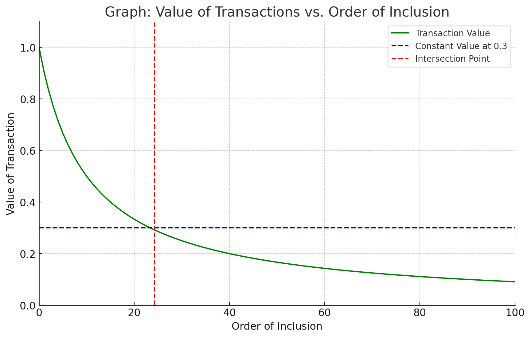
We make the assumption that top of the block gas space is more valuable. The main assumption is that at some point, the marginal value for a builder owning the whole block (green) goes below the marginal value of a beta buyer (typically someone who wants to be just included independently of the order).

If we had perfect information, we could fix the capacity constraint at exactly the intersection point. But this information is not available. We can only approximate it. The question of lottery blocks can also be seen in the diagram, the question is whether for such a block both curves are shifted in the same way. If not, it would indicate the need to give alpha builders more space relative to beta builders. There is another aspect to consider. The larger the alpha part, the larger the possibility of including a txs in beta that will revert (due to state changes). This will degrade the value of the option to buy beta space. What is more, this might jeopardize the service as a whole. If builders get the impression that the service is not of sufficient quality, then they will stop using it. So there is also a reputation component - in particular at the beginning.

Bidder characteristics

Key Assumption

We operate under the assumption that position does not matter; if it does might affect the design significantly.

Bidders are possibly risk-averse, therefore standard revenue equivalence might go out of the window.

• Bidders are asymmetric: in particular if there is private orderflow.

• Bidders valuations are not clear: If they draw from a public mempool or if there are global conditions affecting value of block space, their valuations will be interdependent. - There is also the danger of a further coordination issue; this might favor a winner-takes-all solution.

Relation to the secondary market

Traditionally we would assume that a well-designed auction does not require a secondary market. If the result of the auction is in the core, no change in the allocation makes sense. This is different here as information comes in overtime. BASE_FEE², Transactions updates for alpha bidders We operate under the assumption that position does not matter; if it does might affect the design significantly.

New bidders are active on the secondary market. The secondary market therefore is not just a reallocation of the primary auction but includes information updates.

Important Mechanism Side Effects

This is in contrast to most work on auctions with resale (re: secondary) markets. The secondary market changes the rationale for bidding in the primary auction.

Footnotes

1. Kastl, Jakub. “Discrete Bids and Empirical Inference in Divisible Good Auctions.” Review of Economic Studies 78, no. 3 (2011): 974–1014. ↩

2. BASE_FEE is a lagging indicator, by 6 blocks. ↩